Booting and Managing AWS Redshift Clusters from R

Leaving an AWS Redshift Cluster running all the time can be expensive and unnecessary. It would be nice to be able to efficiently boot, use and shut down a cluster programmatically.  Many times, I’m performing 1-off analyses where my workflow is:

  1. boot up the cluster from a snapshot
  2. aggregate the data in-database and pull into memory using dplyr
  3. shut down the cluster, possibly saving as a snapshot

Thankfully, AWS has a CLI. Using this and some system() magic, we can execute our entire analysis from within R.

# -------------------------------------------------------------
# This script is a proof-of-concept to explore
# connecting to AWS Redshift, identifying a cluster
# snapshot, restoring that cluster, then shutting it down. 
# This is a first step in a package which could help 
# automate some database management tasks
# 
# -Tim Kiely, 9/9/2016
# timothy.j.kiely@gmail.com
# -------------------------------------------------------------

# -------------------------------------------------------------
# Note that you must first set up the aws CLI, see: 
# http://docs.aws.amazon.com/cli/latest/userguide/installing.html
# 
# You will also need to grant access to your user to access
# your Redshift db through IAM settings, see: 
# http://docs.aws.amazon.com/redshift/latest/mgmt/redshift-iam-authentication-access-control.html
# -------------------------------------------------------------


# requries:
library(beepr)
library(dplyr)
library(jsonlite)


# issue an AWS CLI command to list all available Redshift snapshots, catpure as JSON
systext_snapshots <- system("aws redshift describe-cluster-snapshots",intern = T)

# convert the snapshot data from JSON to a dataframe
snapshot_frame <- jsonlite::fromJSON(systext_snapshots)

# Grab the most recent snapshot
most_recent_snap <- dplyr::arrange(snapshot_frame$Snapshots, desc(SnapshotCreateTime)) %>% head(n=1)

# create unique snapshot temp identifier
clust_id <- paste0("cluster-temp-",as.integer(Sys.time()),collapse = "-")

# issue CLI command to create a temp redshift cluster, from the snapshot
restore_command <- paste0("aws redshift restore-from-cluster-snapshot --cluster-identifier ", clust_id," --snapshot-identifier ", most_recent_snap$SnapshotIdentifier)
system(restore_command)


# clusters may take 5-20 minutes to become available. Proceed once the status 

status<-"new"

while(status != "available"){
 cat("Checking...\n")
 Sys.sleep(5)
 systext_check <- jsonlite::fromJSON(system("aws redshift describe-clusters",intern = T), flatten = T)
 
 # extract the correct cluster based on the unique ID:
 systext_check_temp <- dplyr::filter(as.data.frame(systext_check$Clusters), ClusterIdentifier==clust_id)
 
 # set status. if not "available", repeat loop
 status <- systext_check_temp$ClusterStatus
}; beepr::beep(4)

# grab status again
systext_nodes <- jsonlite::fromJSON(system("aws redshift describe-clusters",intern = T), flatten = T)
our_nodes <- filter(systext_nodes$Clusters, ClusterIdentifier == clust_id)

# extract address and port, to be used for querrying
our_nodes$Endpoint.Address
our_nodes$Endpoint.Port


# shut it down!
shut_down_cmd <- paste0("aws redshift delete-cluster --cluster-identifier "
 , our_nodes$ClusterIdentifier
 ," --skip-final-cluster-snapshot")
system(shut_down_cmd)

Once you’ve extracted the Endpoint and Port, you can use dplyr to connect directly to the database for fast, in-db calculations.

Drone Sightings in the US

This is my entry for the new weekly data visualization challenge posted here:

https://rud.is/b/2016/03/30/introducing-a-weekly-r-python-js-etc-vis-challenge/


Main_plot_01


Animated to show concentration over time. Interestingly, at the peak in August 2015, the sightings are relatively concentrated:

DRONES


Where are you most likely to see drones in the US? According to the above maps, we see distinct hot zones in and around NYC, Southern Florida, Texas, and LA. The city of Lost Angels takes the cake, far outpacing even Silicon Valley, which surprised me quite a bit.

Why LA? I know drones are used for highway patrol around SoCal, so maybe that’s it. Or, perhaps, the paparazzi are stepping up their invasion-of-privacy game stalking celebs. Either way, if you’re a drone vendor, here are your target markets!

# Let's make some geo spatial heatmaps with drone data! (no nerds here or anything...)

# set your wd:
setwd("~/Dropbox (Personal)/Viz_Challenges")

library(ggplot2)
library(ggthemes)
library(readxl)
library(dplyr)
library(grid)
library(readr)
library(gplots)

# get copies of the data locally
URL1 <- "http://www.faa.gov/uas/media/UAS_Sightings_report_21Aug-31Jan.xlsx"
URL2 <- "http://www.faa.gov/uas/media/UASEventsNov2014-Aug2015.xls"

fil1 <- basename(URL1)
fil2 <- basename(URL2)

if (!file.exists(fil1)) download.file(URL1, fil1)
if (!file.exists(fil2)) download.file(URL2, fil2)

# read it in
xl1 <- read_excel(fil1)
xl2 <- read_excel(fil2)

# munge it a bit so we can play with it by various calendrical options

drones <- setNames(bind_rows(xl2[,1:3],
 xl1[,c(1,3,4)]),
 c("ts", "city", "state"))
drones <- mutate(drones,
 year=format(ts, "%Y"),
 year_mon=format(ts, "%Y%m"),
 ymd=as.Date(ts),
 yw=format(ts, "%Y%V"))

## to plot on a map, we'll need lat/lon coordinates of US cities
# read in geo lat/lon coordinates by city
# credit to the fine folks at MIT for open-sourcing that!

URL3<-"http://simplemaps.com/files/cities.csv"
fil3 <- basename(URL3)
if (!file.exists(fil3)) download.file(URL3, fil3)
Cities<-read_csv("cities.csv")

# list of states with their abbreviations:
URL4<-"http://www.fonz.net/blog/wp-content/uploads/2008/04/states.csv"
fil4 <- basename(URL4)
if (!file.exists(fil4)) download.file(URL4, fil4)
States<-read_csv("states.csv")

Cities2<-
 left_join(Cities,States,by=c("state"="Abbreviation")) %>%
 mutate("City-State"=paste0(city,"-",State)) %>%
 select(`City-State`,lat,lng,zip)

# looking at drone counts by city
By_City<-
drones %>%
 group_by(year,city,state) %>%
 dplyr::summarise(count=n()) %>%
 mutate("City-State"=paste0(city,"-",state)) %>%
 left_join(Cities2,by="City-State")

# the mapping isn't perfect... how many did we get?
table(is.na(By_City$lat)) # good enough!

## ================ PLOTTING =============== ##
library(ggplot2)
library(grid)
library(gridExtra)

# using ggplot2's map feature
states <- map_data("state")

#draw the base ggplot
ggplot(By_City %>% filter(!is.na(year))) + 

 # add the US map
 geom_polygon(data = states
 ,aes(x = long, y = lat, group = group),
 fill = "grey", color = "black") +

 # plot the drone sightings
 geom_point(aes(x=lng, y=lat, size=count),color="darkred")+

 # add density lines
 stat_density2d(aes(x = lng
 , y = lat)
 ,n=100
 ,size=0.5
 ,bins=10
 ,color="white") + 

 # add a second density layer, this time with color
 stat_density2d(aes(x = lng
 , y = lat
 ,fill=..level..
 ,alpha=..level..)
 ,n=100
 ,size=1
 ,bins = 10
 ,geom = "polygon") + 

 # various theme parameters
 scale_fill_gradient(low = "yellow", high = "red") +
 scale_alpha_continuous(range = c(0.1,0.8))+
 coord_map(xlim=c(-130,-60),ylim=c(23,50))+
 theme_map()+
 theme(legend.position="none"
 ,title=element_text(size=15,face="bold")
 ,panel.background=element_rect(fill="black")
 )+
 labs(title="Where are you most likely to see a drone in the U.S?"
 ,subtitle="Drone sightings in the US; 2014 - 2016"
 ,caption="Data from http://www.faa.gov/uas/law_enforcement/uas_sighting_reports/")


I’ve found that when looking at geospatial data over time, the GIF is a wonderful tool! Let’s make one…


## Draw a GIF!!!

# we'll slice the drone data by month for our GIF (don't want too many panes)
By_month<-
 drones %>%
 mutate(month=lubridate::month(ts,lab=T)) %>%
 group_by(year,month,year_mon,city,state) %>%
 dplyr::summarise(count=n()) %>%
 mutate("City-State"=paste0(city,"-",state)) %>%
 left_join(Cities2,by="City-State") %>%
 ungroup() %>%
 mutate(MonthLab=paste0(month,"-",year))

# some quick munging to make the plot order correct
monthOrder<-
By_month %>%
 group_by(year_mon,MonthLab) %>% summarise(count=sum(count)) %>%
 select(-count) %>%
 filter(!is.na(year_mon)) %>%
 ungroup() %>%
 select(-year_mon)
monthOrder<-as.character(monthOrder$MonthLab)

By_month<-By_month %>% mutate(MonthLab=factor(MonthLab,levels=monthOrder))

# Here's our draw.map function. This will create the main ggplots we
# want in our GIF. We'll make a title, the heatmap, a barplot showing
# what month we're looking at, and then a caption with source info

draw.map<-function(period){

 # 1) The main heatmap. Similar to above
 plot<-
 ggplot(By_month %>% filter(year_mon==period))+

 # add the US map
 geom_polygon(data = states
 ,aes(x = long, y = lat, group = group),
 fill = "grey", color = "black") +

 # plot the drone sightings
 geom_point(aes(x=lng, y=lat, size=count),color="darkred")+

 # add density lines
 stat_density2d(aes(x = lng
 , y = lat)
 ,n=100
 ,size=0.5
 ,bins=5
 ,color="white") + 

 # add a second density layer, this time with color
 stat_density2d(aes(x = lng
 , y = lat
 ,fill=..level..
 ,alpha=..level..)
 ,n=100
 ,size=1
 ,bins = 5
 ,geom = "polygon") + 

 # various theme parameters
 scale_fill_gradient(low = "yellow", high = "red") +
 scale_alpha_continuous(range = c(0.1,0.3))+
 coord_map(xlim=c(-130,-60),ylim=c(23,50))+
 theme_map()+
 theme(legend.position="none"
 ,title=element_text(size=15,face="bold")
 ,panel.background=element_rect(fill="black")
 )

 # 2) adding a nice bar plot below the heatmap so we can see relative volume by month
 bar_plot<-
 By_month %>%
 mutate(color=ifelse(year_mon==period,"current","other")) %>%
 ggplot(aes(x=MonthLab,y=count,group=color,fill=color))+
 geom_bar(stat="identity")+
 geom_vline(xintercept=period,color="red")+
 scale_fill_fivethirtyeight()+
 theme_bw()+
 theme(axis.text.x=element_text(angle=45,hjust=1,size=20)
 ,legend.position="none")+
 xlab(NULL)+ylab(NULL)

 # 3) title
 text<-
 textGrob("Drone Sightings in the US"
 ,gp = gpar(fontsize=30,fontface="bold")
 )

 # 4) caption
 captionText<-
 textGrob("Data from http://www.faa.gov/uas/law_enforcement/uas_sighting_reports/"
 ,gp = gpar(fontsize=20,fontface="italic")
 )

 # arrange everything and play with the height ratios
 grid.arrange(text,plot,bar_plot,captionText,ncol=1,heights=c(0.5,3,0.5,0.5))
}

# we'll need a sequence to run draw.map over
seq<-names(table(By_month$year_mon))

# finally, a second function which just runs the above function
trace.animate <- function() {
 lapply(seq, function(i) {
 draw.map(i)
 })
}

# execute and save the GIF!
library(animation)
saveGIF(trace.animate(), movie.name="DRONES.gif",ani.width = 1400, ani.height = 1400)


If we’re graphing, we’ll need some color palettes


#
cols <- c(“#000000″,”#556670″,”#771C19″,”#8E9CA3″,”#AA3929”, #haloween colors
“#B6C5CC”,”#E25033″,”#E2C59F”,”#F27314″,”#F8A31B”, #haloween colors
“#999999”, “#E69F00”, “#56B4E9”, “#009E73”, #cb firendly colors
“#F0E442”, “#0072B2”, “#D55E00”, “#CC79A7” # cb friendly colors
)

library(scales)
cc <- scales::seq_gradient_pal(“darkgrey”, “skyblue”, “Lab”)(seq(0,1,length.out=12))

Auto-selecting the decision threshold in binary classification

For a while, my default decision threshold for all binary classification tasks was 0.5: Above 0.5 was a 1, below 0.5 was a 0.

The 0.5 threshold provides some stability when comparing one model to another, but really, 0.5 is almost as arbitrary as choosing any number.

So, here are two objective functions for auto-selecting decision thresholds based on different optimization criteria.

The first chooses the apex point on the ROC curve as the cutoff. Good for general purpose models being evaluated by AUC.

The second computes the F-measure, which is a weighted average of precision and recall. The maximum F-measure statistic is taken as the cutoff threshold. This might be used for problems where we are most interested in finding all of our true positives. For example, in “class-imbalance” problems, where the occurrence of an event is rare, such as cancer detection.

# First, we'll create some sample data to simulate a binary classification set.seed(1)
actual <- sample(size=10000 ,c(0,1),replace=T)
predicted <- rnorm( 10000 ,mean=0.5,sd=0.1)

# Let's stack the deck a bit for the predicted values, to make the plots more interesting...
actual <- c(actual,as.integer(predicted>0.55))
predicted<-c(predicted,predicted)

# So now we have our test and control:
summary(predicted)
hist(predicted)

 Min. 1st Qu. Median Mean 3rd Qu. Max. 
0.06972 0.43150 0.49710 0.49840 0.56480 0.87280

Example Pred

summary(as.factor(actual))
 0  1 
12075 7925 
hist(actual)

Actual Example Plot

Now that we have our sample, data, let’s look at optimizing the decision threshold by the apex of the ROC curve:

library(Epi) # To help us vizualize the apex of the ROC curve 

opt<-ROC(predicted, actual ,plot = c("ROC"))
ROC Example
We can see the apex quite clearly. Using the obect we created "opt", we can extract that apex and use it as our decision threshold.
mx <- max(opt$res[, 1] + opt$res[, 2])
mhv <- which((opt$res[, 1] + opt$res[, 2]) == mx)
mxf <- opt$res[["predicted"]][mhv] # note: the name of the predicted values column is set by the user above
print(mxf)
[1] 0.5499367
Next, using the same data, let's extract a different threshold optimizing for the F-measure
https://en.wikipedia.org/wiki/Precision_and_recall#F-measure
library(ROCR) # Used to calculate the F-measure
predROCR = prediction(predicted, actual)
perfROCR = performance(predROCR,"f") #calculates the f measures across cutoffs

# Plot the output, add a red line at the maximum
plot(perfROCR) 
abline(v=PRFMAX,col="red")

F Measure Example
As seen above, the F measure is computed across various cutoffs, with a clear optimal point. Let’s extract that


prfmx<-max(perfROCR@y.values[[1]],na.rm=T) # extracts the max F measure
PRFMAX<-min(perfROCR@x.values[[1]][perfROCR@y.values[[1]]==prfmx],na.rm=T)
print(PRFMAX)

[1] 0.5499544


Record Linkage of Company names

Record linkage is an immensely useful, albeit tedious, task. Easily, one of the most common requests I’ve encountered in an enterprise environment is “wouldn’t it be great to see all of this data from all these different places in the same location?” (AND make it make it predictive, make it interactive, make it into a web app and why doesn’t it look like Microsoft Powerpoint?, and update me on progress every 3 days…). Never mind that these two databases might as well have been developed on different planets: no hard matching key, no consistent data hierarchy, sometimes the only unique identifier is a row number!

Your team: Probably just you, but here are the hats you’ll have to wear:
– Business owner: Defines the problem. Identifies and interviews stakeholders, asks “what would be useful for you and/or where can I get that data?”
– Extraction Team: Works with dev ops / IT of the databases in question to automate access and set up a centralized repository (even if that’s just a local desktop)
– Transformation Team: Ideally, 1 person per database you wish to link. Owns the SQL queries for rolling up data and works with stakeholders to verify the rowcounts are mostly correct (most of the time, nobody ever knows if the rowcounts are exactly correct)
– Linkage modeler: Creates the linkage table. Needs strong data munging skills and should know how to build a classifier
– Reporting Team: researches industry reports, creates top-down list of desired views and works to reconcile with available data
– Visualization Team: because, why do anything if it’s not fun?

Planning and research
If you’re using R, the packages available for this specific problem are somewhat sparse. You have agrep() and adist() for linkage, which both help, but the real problem is one of computation. Consider 12,000 possible names in one database and 115,000 in the other, that’s over a billion possible matches. In addition, how do you define what a match is? How many false positives are you willing to tolerate? See here for some ideas: http://stackoverflow.com/questions/6683380/techniques-for-finding-near-duplicate-records

The RecordLinkage package, which for some reason was archived and abandoned, offers some excellent tools for dealing with the computation issue. The package is the result of work by Murat Sariyar and Andreas Borg, and they lay out some key concepts in this article: http://journal.r-project.org/archive/2010-2/RJournal_2010-2_Sariyar+Borg.pdf

Note: You’ll need to install RecordLinkage from the archive

Key concepts:
– Blocking: the concept of only creating possible match pairs based on some hard criterion, such as only searching for pairs within the group where the first letter of the first word matches. Drastically reduces computation time and effort, and actually increases accuracy (or, more technically, increases precision at the expense of recall, i.e., failing to identify true positives).
– Phonetic functions (e.g., soundex) and string comparison (e.g., levenshein distance): Functions for comparing like strings. Useful if using RecordLinkage for weighting, and can also be very useful when used in conjunction with blocking (i.e., compare this string to all other strings which sound like it)

Before we get to the code, some key learnings:

– Pre-processing is IMMENSELY valuable in this process. Below, the  functions CleanseNames(), SplitNames(), StandardizeWord(), MapFrequency(), and RearrangeWord() are the heart of the pre-processing and cleansing, and are responsible for 80-90% of the matches.

– The ApplyAdist() and ModifyAdist() functions at the bottom can be used to judge relative distances between two character strings

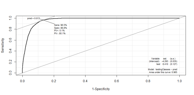
Finally, performance: 

The below code, while heavily obfuscated, achieved an identical match rate to the commercially available D+B service which performs the same task.


#============================================================================
#============================================================================
#================= ENTERPRISE RECORD LINKAGE v.3 ==============================
#============================================================================
#============================================================================
#============================================================================
#============================================================================
# This is my third attempt at the linkage table creation process
# -Tim Kiely
# 8/10/2014
# timothy.j.kiely@gmail.com
#============================================================================

libs <- c("RODBC", "utils", "tm", "stringr", "gdata", "dplyr", "lubridate","beepr")
lapply (libs, library, character.only = TRUE, logical.return=TRUE)

#make sure you've already installed RecodLinkage from the archive
library(RecordLinkage)

#============================================================================
#============================================================================
#===================Pre-Processing for Record Linkage========================
#============================================================================
#============================================================================
#

# First, for both dataframes you wish to merge, create a character string variable called "Company.Name.Compress" which contains names of the companies
# Note: this step cleanses "Company.Name.Compress"
# Also replaces common words, e.g. "INCORPORATION" replaces "INC." and "Inc"
#
#============================================================================

CleanseNames <- function(companies) {
##Remove Special Chars
companies$Company.Name.Compress <- gsub("\\.", "", companies$Company.Name.Compress)
companies$Company.Name.Compress <- gsub("'", "", companies$Company.Name.Compress)
companies$Company.Name.Compress <- gsub("\\ &", " AND ", companies$Company.Name.Compress)
## Convert to UPPER CASE
companies$Company.Name.Compress <- toupper(companies$Company.Name.Compress)
## Remove Stopwords #NOTE: REMOVED THIS STEP: REMOVES IMPORTANT IDENTIFYING INFO AND HINDERS MATCH ABILITY
#companies$Company.Name.Compress <- removeWords(companies$Company.Name.Compress, stopwords("english"))
## Remove Punctuations
companies$Company.Name.Compress <- removePunctuation(companies$Company.Name.Compress)
## Eliminating Extra White Spaces
companies$Company.Name.Compress <- stripWhitespace(companies$Company.Name.Compress)
## Eliminate leading White Space
companies$Company.Name.Compress <- gsub("^ ", "",companies$Company.Name.Compress)
## Eliminate trailing White Space
companies$Company.Name.Compress <- gsub(" $", "", companies$Company.Name.Compress)
## Remove Numbers
#companies$Company.Name.Compress <- removeNumbers(companies$Company.Name.Compress)
return(companies)
}

df.companies.cleansed <- CleanseNames(df.companies)
df.db.companies.cleansed <- CleanseNames(df.db.companies)

#============================================================================
#============================================================================
#========================= WORD REPLACEMENT =================================
#============================================================================
#============================================================================
#
# Splits the company names and stores the first 5 words in seperate variables.
# If the name has less then 5 words then the remaining words are
# automatically assigned NA
#
# Note: this is the most time-consuming preprocessing operation
# (excluding record linkage, which is computationally expensive)
#
# If optimization is desired, this function could be improved
#
#============================================================================
SplitNames <- function(companies){
companies <- data.frame(companies
,First.Word= NA
,Second.Word= NA
,Third.Word= NA
,Fourth.Word= NA
,Fifth.Word= NA
,stringsAsFactors=F)


companies <- companies %.% group_by(1:n()) %.%
mutate(LinLen = length(unlist(strsplit(Company.Name.Compress," ")))
,First.Word = ifelse(LinLen<1,"",toupper(word(Company.Name.Compress,1)))
,Second.Word = ifelse(LinLen<2,"",toupper(word(Company.Name.Compress,2)))
,Third.Word = ifelse(LinLen<3,"",toupper(word(Company.Name.Compress,3)))
,Fourth.Word = ifelse(LinLen<4,"",toupper(word(Company.Name.Compress,4)))
,Fifth.Word = ifelse(LinLen<5,"",toupper(word(Company.Name.Compress,5)))
)
return(companies)
}

df.companies.split <- SplitNames(df.companies.cleansed)
df.db.companies.split <- SplitNames(df.db.companies.cleansed)
#============================================================================
#============================================================================
#========================== WORD STANDARDIZATION ============================
#============================================================================
#============================================================================
#
# Replaces Common interchangable words with standards, e.g.:
# "INCORPORATED" replaces "INC" and "Inc.", etc.
#
# Also, importantly creates the "Full.String" variable (concat of 5 words)
#
#============================================================================
StandardizeWord <- function (companies){

companies <- as.matrix(companies)

# Initial words are replaced by Final Words
initial <- c("CORP","USA","INC","CO","LTD","INTL","COMP","SVCS","SERVICE","HLDGS","MORTG","SYS","TECH",
"IND","SERV","FINL","LABS","TELECOMMUN","MTG","CP","PPTYS","SEC","COMMUN","DIST", "INCORPORATED",
"COS", "CORPO", "CORPOR", "CORPORA", "CORPORATI", "CORPORAT", "CORPORATIO", "CORPORATIONS",
"HLTHCR")

final <- c("CORPORATION","US","INCORPORATION","COMPANY","LIMITED","INTERNATIONAL","COMPANY","SERVICES",
"SERVICES","HOLDINGS","MORTGAGE","SYSTEM","TECHNOLOGY","INDUSTRIES","SERVICES", "FINANCIAL",
"LABORATORIES","TELECOMMUNICATIONS","MORTGAGE","CORPORATION","PROPERTIES","SECURITIES",
"COMMUNICATIONS","DISTRIBUTION", "INCORPORATION", "CORPORATION", "CORPORATION", "CORPORATION",
"CORPORATION", "CORPORATION", "CORPORATION", "CORPORATION", "CORPORATION", "HEALTHCARE")
word.standard <- as.matrix(cbind(initial, final)) # Creating a data.frame


# running the loop over the five words
var <- c("First.Word", "Second.Word", "Third.Word", "Fourth.Word", "Fifth.Word")
for(i in 1:5){
match.index <- match(companies[, var[i]], word.standard[,"initial"])
companies[, var[i]] <- ifelse(!is.na(match.index), word.standard[,"final"][match.index], companies[, var[i]])
}


# Creating a standardized full name again, by pasting back the five words
companies <- data.frame(companies, Full.String="NA")

companies <- companies %.%
group_by(1:n()) %.% mutate(Full.String=trim(paste(First.Word
, Second.Word
, Third.Word
, Fourth.Word
, Fifth.Word)
)
,Full.String=gsub("NA","",Full.String)
)
companies <- as.data.frame(companies,stringsAsFactors=F)
return(companies)
}
df2.companies <- StandardizeWord(df.companies.split)
df2.db.companies <- StandardizeWord(df.db.companies.split)
#============================================================================
#============================================================================
#========================== WORD SIGNIFICANCE CALC ==========================
#============================================================================
#============================================================================
#
# Calculate most significant word
# "INCORPORATED" replaces "INC" and "Inc.", etc.
#
# Also, importantly creates the "Full.String" variable (concat of 5 words)
#
#============================================================================
var <- c("First.Word","Second.Word","Third.Word","Fourth.Word","Fifth.Word")
words<-matrix()
db.words<-matrix()
words<-c(as.matrix(df2.companies[,var]))
words<-as.data.frame(words[!is.na(words)])
db.words<-c(as.matrix(df2.db.companies[,var]))
db.words<-as.data.frame(db.words[!is.na(db.words)])
names(words)="words"
names(db.words)="words"
words<-rbind(words,db.words)
freq.table<-words%.%group_by(words)%.%summarise(count=n())%.%arrange(-count)
freq.table <- as.matrix(freq.table)
# renaming the columns of frequency table
colnames(freq.table)[1] <- "Word"
colnames(freq.table)[2] <- "Freq"

MapFrequency <- function(companies, frequencies){

var <- c("First.Word", "Second.Word", "Third.Word", "Fourth.Word", "Fifth.Word")

# running the loop over 5 words
for(i in 1:5){
# renaming column name of "frequencies" to Freq.Word1, Freq.Word2 etc. in each iteration
colnames(frequencies)[2] <- paste("Freq.Word", i, sep="")

# merging Freq.Word1 for var[1] i.e. "First.Word" ; Freq.Word2 for var[2] i.e. "Second.Word" and so on..
companies <- as.matrix(merge(companies, frequencies, by.x=var[i], by.y="Word", all.x=TRUE))
}

companies <- as.data.frame(companies)
return(companies)
}
df2.companies <- MapFrequency(df2.companies,freq.table)
df2.db.companies <- MapFrequency(df2.db.companies,freq.table)
#=======================================================================================
# RearrangeWord
#
# Purpose: Rearrange the individual word columns and respective frequency columns as
# least frequent to most frequent from left to right. Word having the least
# frequency is most significant.
#
# Arguments:
# db.companies: A matrix having the individual word columns and the respective
# frequency columns
#
# Returns:
# A matrix with rearranged individual word columns according to their significance
#=======================================================================================
RearrangeWord <- function(db.companies){
as.matrix(db.companies)

var2 <- c("Freq.Word1", "Freq.Word2", "Freq.Word3", "Freq.Word4", "Freq.Word5")
var <- c("First.Word", "Second.Word", "Third.Word", "Fourth.Word", "Fifth.Word")

numeric.sorting <- function(temp) order(as.numeric(as.matrix(temp)))

# applying the sort function row wise
ordering.index <- apply(as.matrix(db.companies[, var2]), 1, numeric.sorting)

# correcting the ordering.index.
# It is actually a linear vector (not a matrix) and hence need to be corrected
ordering.index <- ordering.index + 5 * (col(ordering.index)-1)

# Rearranging the word frequencies
db.companies[,var2] <- t(matrix(t(db.companies[, var2])[ordering.index], nrow = 5, ncol = nrow(db.companies)))

# Rearranging the words themselves
db.companies[, var] <- t(matrix(t(db.companies[, var])[ordering.index], nrow = 5, ncol = nrow(db.companies)))

# Renaming the words
colnames(db.companies)[match(var, colnames(db.companies))] <- c("Sig.Word1", "Sig.Word2",
"Sig.Word3", "Sig.Word4", "Sig.Word5")
as.data.frame(db.companies)
return(db.companies)
}
df2.companies <- RearrangeWord(df2.companies)
df2.db.companies <- RearrangeWord(df2.db.companies)
#============================================================================
#============================================================================
#================ RECORD LINKAGE FEATURE SELECTION ==========================
#============================================================================
#============================================================================
#
# Re-Extracting the First Word, Second Word etc. features for improved blocking
df2.companies$Company.Name.Compress<-as.character(df2.companies$Company.Name.Compress)
df2.db.companies$Company.Name.Compress<-as.character(df2.db.companies$Company.Name.Compress)
df.companies.extra <- SplitNames(df2.companies)
df.db.companies.extra <- SplitNames(df2.db.companies)
#
df2.companies <- df.companies.extra
df2.db.companies <- df.db.companies.extra

#
#============================================================================
df2.companies$companies <- as.factor(df2.companies$companies)
df2.companies$Company.Name.Compress <- as.factor(df2.companies$Company.Name.Compress)
df2.companies$First.Word <- as.factor(df2.companies$First.Word)
df2.companies$Second.Word <- as.character(df2.companies$Second.Word)
df2.companies$Third.Word <- as.character(df2.companies$Third.Word)
df2.companies$Fourth.Word <- as.character(df2.companies$Fourth.Word)
df2.companies$Fifth.Word <- as.character(df2.companies$Fifth.Word)
df2.companies$Full.String <- as.character(df2.companies$Full.String)
df2.companies$LinLen <- as.integer(df2.companies$LinLen)
df2.companies$employer_key <- as.integer(df2.companies$employer_key)
df2.companies$Sig.Word1 <- as.factor(df2.companies$Sig.Word1)

df2.db.companies$db.companies <- as.factor(df2.db.companies$db.companies)
df2.db.companies$Company.Name.Compress <- as.factor(df2.db.companies$Company.Name.Compress)
df2.db.companies$First.Word <- as.factor(df2.db.companies$First.Word)
df2.db.companies$Second.Word <- as.character(df2.db.companies$Second.Word)
df2.db.companies$Third.Word <- as.character(df2.db.companies$Third.Word)
df2.db.companies$Fourth.Word <- as.character(df2.db.companies$Fourth.Word)
df2.db.companies$Fifth.Word <- as.character(df2.db.companies$Fifth.Word)
df2.db.companies$Full.String <- as.character(df2.db.companies$Full.String)
df2.db.companies$LinLen <- as.integer(df2.db.companies$LinLen)
df2.db.companies$Sig.Word1 <- as.factor(df2.db.companies$Sig.Word1)
df2.companies["X1.n.."]<-NULL
df2.companies["X1.n...1"]<-NULL
df2.companies["1:n()"]<-NULL
df2.db.companies["X1.n.."]<-NULL
df2.db.companies["X1.n...1"]<-NULL
df2.db.companies["1:n()"]<-NULL

df2.companies<-as.data.frame(df2.companies)
df2.db.companies<-as.data.frame(df2.db.companies)
table1<- df2.companies%.%select(companies=companies
,Company.Name.Compress
,First.Word
,Sig.Word1
,LinLen
,employer_key)

table2 <- df2.db.companies%.%select(companies=db.companies
,Company.Name.Compress
,First.Word
,Sig.Word1
,LinLen
)%.%
mutate(employer_key=as.integer(seq_along(companies)))
#============================================================================
#============================================================================
#================ RECORD LINKAGE: ===========================================
#================ MATCH PAIR GENERATION =================================
#============================================================================
#============================================================================
#
# Two additional functions for modifying and applying the base approximate distance function adist
# Modified verison "ModifyAdist" penalizes for incorrect first letter and increases penalty for substitutions (decreases chance of false positive)

ApplyAdist <- function(word1, word2){
tryCatch({
ged.string <- adist(word1, word2, counts = T,ignore.case=T)
# Assigning distinct weightages
ged <- sum(attr(ged.string, "counts"))
return(ged)
})
}

#
#

ModifyAdist <- function(word1, word2){
tryCatch({

ged.string <- adist(word1, word2, counts = T,ignore.case=T)
# Assigning distinct weightages
ged <- sum(attr(ged.string, "counts")* c(1, 1, 5))
# 1: Insertion 2: Deletion 3: Substitution

# Adding extra cost if the first character of the string differs
if(strsplit(attr(ged.string, "trafos"), split = "")[[1]][1] != "M") ged <- ged + 8
return(ged)
})
}

#
#
#
#============================================================================
#============================================================================

system.time({

# use this if you want to test on a subset:

tam.frac <- sample_frac(table1,1,replace=F)
db.frac <- sample_frac(table1,1,replace=T)

identity.tam <- as.numeric(tam.frac$employer_key)
identity.db <- as.numeric(db.frac$employer_key)

results <- RLBigDataLinkage(
dataset1 = tam.frac
,dataset2 = db.frac
,identity1 = identity.tam
,identity2 = identity.db
,blockfld = "First.Word"
,exclude = c("companies"
,"employer_key"
,"LinLen"
,"Sig.Word1"
,"First.Word")
,strcmp = "Company.Name.Compress"
,strcmpfun = "levenshtein"
#,phonetic = ""
#,phonfun = "pho_h"
)
})

results.fin <-
getPairs(
results
#,filter.match = c("match", "unknown", "nonmatch")
#,filter.link=c("link")
,max.weight = Inf
,min.weight = -Inf
#,withMatch=T
#,withClass=T
,single.rows=T
)

results.fin$Company.Name.Compress.1<-as.character(results.fin$Company.Name.Compress.1)

results.fin <- results.fin %.%
group_by(1:n()) %.%
mutate(NumChar = length(unlist(strsplit(Company.Name.Compress.1,""))))%.%
mutate(company_aDist = ApplyAdist(companies.1,companies.2)) %.%
mutate(company_MaDist = ModifyAdist(companies.1,companies.2)) %.%
mutate(cleansed_aDist = ApplyAdist(Company.Name.Compress.1,Company.Name.Compress.2)) %.%
mutate(cleansed_MaDist = ModifyAdist(Company.Name.Compress.1,Company.Name.Compress.2)) %.%
mutate(Clnsd_dist_over_len = cleansed_MaDist/NumChar)%.%
arrange(cleansed_MaDist)
results.fin$SD_MaD <- scale(results.fin$cleansed_MaDist)
results.fin$SD_DoL <- scale(results.fin$Clnsd_dist_over_len)

&nbsp;


Working from home? Auto-detect which computer you are working from

I carry my projects back and forth from work to home. Ideally, developing in a cloud environment, such as GitHub, would be great. But in reality, my projects for work don’t allow me to post code or data to the cloud (we do have a shared drive, but connecting to the VPN can be a pain…).

My somewhat hack-ish solution has been to use an external drive to ferry my projects back and forth. As a kind of pre-Victorian version control, I’l periodically upload the project folders to the shared drive like a new commit (e.g., “Project_Folder_03_09_2015.zip”).

Reducing friction between developing in one environment to the next is necessary, so I’ve come up  with a simple way to detect the computer you are currently plugged into. This allows me to plug in an external drive and with minimal touch, detect the current computer and set the correct working environment.


The trick is using the Sys.getenv() function, which returns a while host of environment information when called. The variable we are interested in is “COMPUTERNAME”:

# FROM my LAPTOP:
 if(Sys.getenv()["COMPUTERNAME"]=="0000-0000000"){
 setwd("D:/MyPath/Project")

# FROM my DESKTOP:
 } else if(Sys.getenv()["COMPUTERNAME"]=="9999-9999999"){
 setwd("F:/MyPath/Project")

} else stop("This machine is not recognized.
 \nAdd a working directory to the beginning of SCRIPT.R")

You can of course continue to add new “COMPUTER NAMES” as needed. Extending this to an automated, user-input type interface would be trivial… which could be useful for local deployment of, say, Shiny Apps or the like.

Copy/Paste data in and out of R

Imagine moving data in and out of R as easily as with Excel/Powerpoint/Outlook via the ctrl+c/ctrl+v commands. Turns out you can.

For business analyst jobs, summarizing and communicating data rapidly is a daily necessity. If you happen to communicate data to people primarily via Microsoft Excel/Powerpoint/Outlook (you shouldn’t, but let’s face it, it comes up a lot), the following tip is invaluable.

How to copy data in and out of R using the clipboard

Disclaimer: have not tried this in a Mac OS or Linux environments.

Imagine, for example, our teammate desperately needed to know the average mpg for different numbers of cylinders in the mtcars data set. Easy, we think, using dplyr:


> mtcars %>% group_by(cyl) %>% summarise(MEAN_MPG=mean(mpg))
Source: local data frame [3 x 2]

  cyl MEAN_MPG
1   4 26.66364
2   6 19.74286
3   8 15.10000

For a long time, regardless of the size of the dataframe, I would move data in and out of R by reading and writing data to and from a .csv. But the above output is a table of trivial size, not worth the incremental clutter created by writing to a .csv. Instead, let’s simply copy and paste that bad boy using write.table()

OurData <- 
mtcars %>%
  group_by(cyl) %>%
  summarise(MEAN_MPG=mean(mpg))

write.table(OurData,"clipboard",sep="\t",row.names=F)

That works! In write.table(), specify the destination file as “clipboard” and use sep=”\t” to make tab delimited. Then move it to Excel, Powerpoint or Outlook using ctrl+v.

Note: R has a built-in function called writeClipboard(), but it only accepts character vectors. I find write.table() to be friendlier and with finer control. Plus, the typing is minimal enough to obfuscate the need for a wrapper, IMO.

On the subject of reducing clutter, we should also strive to keep our R workspaces as clean as possible. Let’s bypass the need to create a new variable (OurData, above).

The %>% or “pipe” operator comes from the magrittr package and is included as part of dplyr. It’s a simple but brilliant operator which takes the dataframe from the left side of the argument and feeds it as the first argument in the following function. It’s the reason why dplyr can be written in the order of thought, rather than having to nest functions. Useful in conjunction with head(), View() and a host of other functions.

Cleaning up the above:


mtcars %>%
  group_by(cyl) %>%
  summarise(MEAN_MPG=mean(mpg)) %>%
  write.table("clipboard",sep="\t",row.names=F)

No need to create a new variable in the R workspace; take the data, perform an operation and save the output directly to the clipboard. Crisp.

The reverse works as well. Copy some data from Excel to the clipboard and read it into R:

data<-read.table("clipboard",sep="\t")

Hope this helps. Enjoy!

Installing RecordLinkage from the archive

Working to achieve database linkage using approximate or “fuzzy” matching, I needed to link customer names in one database to possible matches in another. Fuzzy matching one name to a small list of other possible names is well-documented and actually quite simple in R with agrep() and adist(). The challenge compounds on itself, though, as the list of potential matches grew. I need to match 12K names against a potential list of ~115,000 names–over a billion possibilities. Computation was an issue, especially under tight time constraints.

The package RecordLinkage, by Murat Sariyar and Andreas Borg, attempts to solve this problem in R by implementing the matching using the ff data classes (among many other useful utilities). For some reason I don’t know, RecordLinkage as a project was abandoned and archived. The package still works (and the work is fascinating: http://journal.r-project.org/archive/2010-2/RJournal_2010-2_Sariyar+Borg.pdf).

To install RecordLinkage from CRAN archive, follow instructions here:
http://stackoverflow.com/questions/24194409/how-do-i-install-a-package-that-has-been-archived-from-cran

On windows, it requires first installing RTools, then running this code:

url <- "http://cran.r-project.org/src/contrib/Archive/RecordLinkage/RecordLinkage_0.4-1.tar.gz"
pkgFile <- "RecordLinkage_0.4-1.tar.gz"
download.file(url = url, destfile = pkgFile)

# Install dependencies

install.packages(c("ada", "ipred", "evd"))

# Install package
install.packages(pkgs=pkgFile, type="source", repos=NULL)

# Delete package tarball
unlink(pkgFile)

Using a “Slope Graph” to Visualize Predicted Rank vs. Actual

“Slope Graphs” are gaining some popularity thanks to Edward Tufte: http://www.edwardtufte.com/bboard/q-and-a-fetch-msg?msg_id=0003nk

An Example of Edward Tufte's "Slope Graph"

An Example of Edward Tufte’s “Slope Graph”

ggplot2 makes Slope Graphs easy to plot via the geom_path() function.

The below code plots rounds 1, 2 and 3 of the 2012 Masters tournament, scraped from ESPN.com at the time of the competition on a Slope graph. Note that I’ve displayed the information quantitatively, i.e., the golfer’s actual scores over the 3 Rounds. This doesn’t align with the spirit of the Slope graph, which is better for qualitative views of data. In a future version it would be better to calculate relative rank on each day, then display the change. It works out OK here because golf scores seem to remain within a relatively stable range.


library(reshape)
library(ggplot2)

Data.masters=structure(list(PLAYER = structure(1:3, .Label = c("Round 1",
"Round 2", "Round 3"), class = "factor"), Marc.Leishman = c(66L,
66L, 69L), Fred.Couples = c(68L, 71L, 73L), Jim.Furyk = c(69L,
69L, 70L), Tiger.Woods = c(70L, 70L, 71L), Angel.Cabrera = c(71L,
69L, 68L), John.Senden = c(72L, 72L, 67L), Adam.Scott = c(69L,
72L, 78L), Jason.Dufner = c(72L, 69L, 64L), David.Lynn = c(68L,
73L, 71L), Lee.Westwood = c(70L, 70L, 80L), Justin.Rose = c(70L,
70L, 70L), K.J..Choi = c(70L, 70L, 74L), Rickie.Fowler = c(68L,
68L, 76L), Jason.Day = c(70L, 70L, 73L)), .Names = c("PLAYER",
"Marc.Leishman", "Fred.Couples", "Jim.Furyk", "Tiger.Woods",
"Angel.Cabrera", "John.Senden", "Adam.Scott", "Jason.Dufner",
"David.Lynn", "Lee.Westwood", "Justin.Rose", "K.J..Choi", "Rickie.Fowler",
"Jason.Day"), row.names = c(NA, 3L), class = "data.frame")

df.set.m <- melt(Data.masters, id.var = c("PLAYER"))

ggplot(df.set.m, aes(PLAYER, value, group = variable)) +
theme(panel.background = element_rect(fill = 'white', colour = NULL)
,panel.grid.major = element_line(color="white")
,panel.grid.minor = element_line(color="white")) +
scale_x_discrete(expand = c(0, 0))+
geom_path(lineend="round",aes(color=variable
#,size=.5
#,alpha=Change
)
)+
xlab(NULL) +
ylab("Rank") +
ggtitle("Predicted Rank vs. Actual Rank")

SlopeGraphExampleMasters

An interesting annotation: it seems that the first day of golf has relatively less variance in scores than the last day. Notice how in Round 3, the scores really start to separate. This could also be due to some occurrence that day (i.e., weather), but the graph at least suggests that in order to do well in the masters, consistency and momentum play a role.

A few more examples, here plotting Predicted Rank of a GBM model vs. Actual Rank:

SlopeGraphExampleRedBlack

Dual ggplot2: different chart, same y-axis

The idea here was to append a density plot to the left of my main plot (an area-rectangle plot in this case. Side note, need to find a better name for that).

dualggplotExampleImage

It was easy enough to generate both plots, but concatenating them was a challenge. I found this very well-written stackoverflow question on the topic: http://stackoverflow.com/questions/14743060/r-ggplot-graphs-sharing-the-same-y-axis-but-with-different-x-axis-scales

Seemed like gridExtra::grid.arrange() was the best way to go rahter than ggplot’s facet_wrap or facet_grid (given that I wanted the two charts to have different widths). I was able to plot the two graphs next to one another with the right spacing, but getting them to share a common y-axis was a challenge. I needed better control over the graphing parameters. I posted the question to stackoverflow: http://stackoverflow.com/questions/24765686/plotting-2-different-ggplot2-charts-with-the-same-y-axis

Turns out ggplot_gtable was exactly what I needed. From ?ggplot_gtable help text: “This function builds all grobs necessary for displaying the plot, and stores them in a special data structure called a gtable. This object is amenable to programmatic manipulation, should you want to (e.g.) make the legend box 2 cm wide, or combine multiple plots into a single display, preserving aspect ratios across the plots.”

Fully reproducible example:

rm(list=ls())
library(ggplot2)
library(gridExtra)
library(dplyr)

df<-structure(list(ratio = c(0.442, 0.679, 0.74, 0.773, 0.777, 
                                 0.8036, 0.87, 0.871, 0.895, 0.986, 1.003, 1.2054, 1.546, 1.6072
), width = c(4222L, 14335L, 2572L, 2460L, 1568L, 8143L, 3250L, 
             17119L, 3740L, 3060L, 2738L, 1L, 1L, 790L)
, w = c(4222L, 18557L, 21129L, 23589L, 25157L, 33300L, 36550L, 53669L, 57409L, 60469L
        , 63207L, 63208L, 63209L, 63999L)
, wm = c(0L, 4222L, 18557L, 21129L
         , 23589L, 25157L, 33300L, 36550L, 53669L, 57409L, 60469L, 63207L, 
         63208L, 63209L)
, wt = c(2111, 11389.5, 19843, 22359, 24373, 29228.5, 
         34925, 45109.5, 55539, 58939
         , 61838, 63207.5, 63208.5, 63604) 
, mainbuckets = c(" 4,222", "14,335", " 2,572", " 2,460", " 1,568", 
                " 8,143", " 3,250", "17,119", " 3,740", " 3,060", " 2,738", 
                "", "", "   790")
, mainbucketsULR = c("0.44", "0.68", "0.74"
                     , "0.77", "0.78", "0.80", "0.87", "0.87", "0.90", "0.99", "1.00", 
                     "", "", "1.61"))
, .Names = c("ratio", "width", "w", "wm", 
             "wt", "mainbuckets", "mainbucketsULR")
, class = c("tbl_df", "tbl", 
"data.frame"), row.names = c(NA, -14L))

textsize<-4

p1<-
  ggplot(df, aes(ymin=0)) + 
  geom_rect(aes(xmin = wm, xmax = w, ymax = ratio, fill = ratio)) +
  scale_x_reverse() +
  geom_text(aes(x = wt, y = ratio+0.02, label = mainbuckets),size=textsize,color="black") +
  geom_text(aes(x = wt, y = 0.02, label = mainbucketsULR),size=textsize+1,color="white",hjust=0,angle=90) +
  xlab("Frequency") +
  ylab("Ratio") +
  ggtitle(paste("My Title")) +
  theme_bw() +
  theme(legend.position = "none"
        ,axis.text.x=element_blank())


p2<-ggplot(df, aes(ratio,fill=width,ymin=0)) + geom_density(color="grey",fill="grey") +
  ggtitle("Density") +
  xlab("") +
  ylab("") +
  theme_bw() +
  coord_flip()+
  scale_y_reverse() +
  theme(text=element_text(size=10)
        ,axis.text.x=element_blank()
        ,legend.position="none"
        #,axis.text.y=element_blank()
  )


limits <- c(0, 2)
breaks <- seq(limits[1], limits[2], by=.5)

# assign common axis to both plots
p1.common.y <- p1 + scale_y_continuous(limits=limits, breaks=breaks)
p2.common.y <- p2 + scale_x_continuous(limits=limits, breaks=breaks)

# At this point, they have the same axis, but the axis lengths are unequal, so ...

# build the plots 
p1.common.y <- ggplot_gtable(ggplot_build(p1.common.y))
p2.common.y <- ggplot_gtable(ggplot_build(p2.common.y))

# copy the plot height from p1 to p2
p2.common.y$heights <- p1.common.y$heights

grid.arrange(p2.common.y,p1.common.y,ncol=2,widths=c(1,5))

Posted the above to github here: https://github.com/timkiely/dualggplot

Much thanks to Matthew Plourde for the stackoverflow answer.

Update: Just looked up “variable width bar charts” and, though there is some confusion/disagreement, this appears to be known as a “Cascade Chart”. Cool.